Jon E. Wallevik

Description of fluid (what is a fluid?)

This text concern the explanation of why large particle systems (with dry or wet particles), like fresh concrete, rings of Saturn or sea ice floes, can be treated as a fluid with the same fundamental properties as for example water. Please click here to download.

Thixotropy and microstructure-rheology (VVPF 3.x)

The material model used in Viscometric-ViscoPlastic-Flow 3.x is named the PFI-theory (Mark II). The theory consists of system of coupled partial differential equations (PDEs). The model has quite many material parameters which are not directly observable and hence are generally unknown. VVPF 3.x has a search module that can automatically retrieve the values of these model parameters. This is done by combining computational fluid dynamics (CFD) with a certain statistical tool, called the direct search method [2]. The overall algorithm solves an optimization problem, in which the difference between the observed data and the output of the PDEs is minimized.

Automatic parameter identification of linear algebraic equation is straightforward, where equation like y = ax + b is fitted to the observed data. That is, through the method of least squares for example, the parameters a and b are easily extracted. However, automatic parameter identification of system of PDEs is much more challenging, basically because there is generally no algebraic solution to the equations. That is, there exist only numerical solutions to the PDEs. Also, the problem of parametric identification is generally difficult due to both the number of parameters that a model can rely on and due to the nonlinear behavior of the governing PDEs. In vvpf 2.0 and 1.0 (see [3,4]), such parameter identification was done manually, where all values were extracted by the means of manual trial and error. That is, all values were manually changed by a computer operator, until the computed data more or less overlapped the measured data. Since automatic parameter identification can play a key role in examining the validity of a complex material model, the generality of the current work is beyond the specific model presented in vvpf 3.x.

BIBLIOGRAPHY

1. Unpublished!
2. J.E. Wallevik, Rheological properties of cement paste: thixotropic behavior and structural breakdown, Cement and Concrete Research, 39 (2009) 14 - 29.
3. J.E. Wallevik, Method of Retrieving the Herschel-Bulkley Parameters When Using the (Wide-Gap) Coaxial Cylinders Viscometer, The Third North American Conference on the Design and Use of Self-Consolidating Concrete, November 10-12, 2008, Chicago, IL.
4. J.E. Wallevik, Thixotropic investigation on cement paste: experimental and numerical approach, J. Non-Newtonian Fluid Mech. 132 (2005) 86 - 99.

Thixotropy and microstructure-rheology (VVPF 2.0)

The material model used in Viscometric-ViscoPlastic-Flow 2.0 is named the PFI-theory (Mark I) and consists of system of coupled partial differential equations (PDEs). In the earlier work (vvpf 1.0), the material model was only thixotropic in origin, based on several ideas proposes by Hattori and Izumi. With a purely thixotropic characteristic, the model was only partly successful. In the model present in vvpf 2.0, however, a certain time-dependent and non-thixotropic process, called structural breakdown is allowed to occur simultaneously with the thixotropic behavior. The combination of the two processes produces a much better result. The concept of structural breakdown is from previous work done by Tattersall and Banfill.

In most cases, when modeling a thixotropic material model, the experiment is based on a very simple shear rate condition. For example, it is popular to apply only one constant angular velocity to the rotating part of the viscometer. In so doing, one can often fit a simple exponential decay of shear rate multiplied by time, with the measured data. Such approach is not done here. More precisely, a much more complicated shear rate condition is applied, which calls for a deeper physical model.

BIBLIOGRAPHY

1. J.E. Wallevik, Rheological properties of cement paste: thixotropic behavior and structural breakdown, Cement and Concrete Research, 39 (2009) 14 - 29.

Thixotropy and microstructure-rheology (VVPF 1.0)

Motivation:

This project consists of measuring and modeling thixotropic behavior of cement paste. More precisely, the project is about the development of a material model (i.e. shear viscosity equation η) for cement paste that can describe its thixotropic behavior under complex shear rate condition. The cement paste is a suspension of cement particles in water. As such, the present theory can be interesting for scientists working with other type of suspensions, like paint.

The main motivations for this project are as follows:

1. Connecting rheological behavior of cement paste to its microstructural state. In so doing, identify and understand one of the key causes for thixotropy and workability loss of the cement based material.
2. Such fundamental understanding can be a valuable tool, for example when choosing a suitable cement type and/or admixture type to be used for a given application at building site.

Note that shear viscosity is also known as apparent viscosity. The reason for that I like the term shear viscosity better, is because it descries what it stands for; i.e. it describes the fluid particles (CP) resistance against shearing deformation. As such, this term reminds us that other types of viscosities also exist like the bulk viscosity and the uniaxial extensional viscosity. The two latter apply for different types of deformations, which are not relevant for this project.

The mathematical approach:

The mathematical approach used in this project consists of computing the flow inside the ConTec Viscometer 4, by solving the governing equation. The computed results are then compared with the experimental results from cement pastes. The computed flow is calculated through the governing equation shown below.

The constitutive equation and the rate-of-deformation tensor are given by the following two equations:

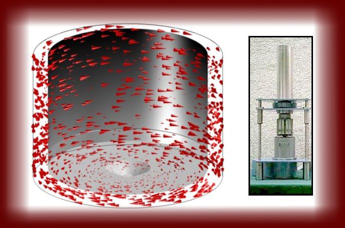
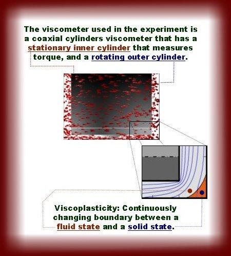
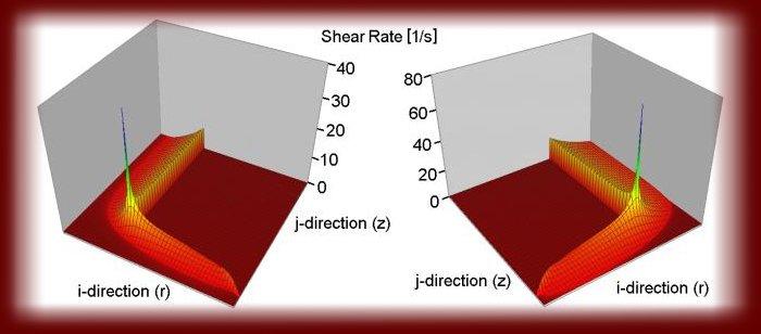
See nomenclature for description of each variable. In the figure below is shown the computed flow inside the ConTec Viscometer 4 (to the left). The viscometer is shown to the right. It has a stationary inner cylinder that measures torque and a rotating outer cylinder (consisting of a bucked). In the left illustration, the direction of the velocity is shown with cones. Larger cones means larger speed and vise versa (speed = absolute value of the velocity). Obviously, since it is the outer cylinder that rotates and the inner cylinder (gray color) that is stationary, the largest cones are near the outer cylinder.

As will be clear below, the material model used in this project is of viscoplastic nature. This means that some part of the solution domain (i.e. some part of the fluid) can be in a solid state (meaning rigid body motion). For time dependent material, the boundary between the fluid state and the solid state is constantly changing inside the viscometer. In the figure below, the orange part demonstrate the solid state and the white part the fluid state. The blue lines are isolines of the speed.

The material model:

In the quest of reproducing the measured torque by numerical means, it became necessary to include yield value into the shear viscosity equation. Both a classical yield value and a thixotropic yield value had to be introduced. In so doing, the material model is of viscoplastic nature and hence some part of the solution domain (i.e. some part of the fluid) can be in a solid state (see the above figure). The shear viscosity and the shear rate are calculated by the following equations:

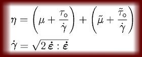
See nomenclature for description of variables. The shear rate equation dates back to Oldroyd (1947). From this equation, it is clear that shear rate is not only dependent on the geometry and angular velocity of the viscometer, but also on the rheological parameters of the test material. This is because of how the shear rate is dependent on the rate-of-deformation tensor, which again is dependent on velocity, which again is calculated by the governing equation. Through the constitutive equation, the governing equation uses information about the rheological parameters of the test material.

[ In the last-mentioned nomenclature, I use the term "yield value" instead of "yield stress". Please note that in the British Standard BS 5168:1975 "Glossary of rheological terms" it is stated that those two terms are the same. ]

Microstructural approach:

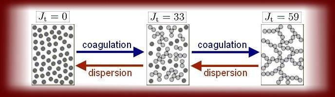
The microstructural approach is based on the previous work done by Hattori and Izumi. More precisely, the coagulation rate and dispersion rate of the cement particles are assumed to play the dominating role in generating thixotropic behavior.

The term coagulation describes the occurrence when two (or more) cement particles come into a contact with each other for some duration of time; i.e. when the cement particles become glued to each other and work is required to separate them (i.e. disperse them). The particles become glued together as a result of the total potential energy interaction that exists between them. This potential energy results from combined forces of van der Waals attraction, electrostatic repulsion and the so-called steric hindrance. For further readings about these forces, see for example Chapter 2.5.2 (p.38) in my Ph.D. thesis (see the link page, about the download location). In this project, it is assumed that there are basically two kinds of coagulation. The first type is the reversible coagulation, where two coagulated cement particles can be separated (i.e. dispersed) again for the given rate of work available to the suspension (the rate of work, or power, is provided by the engine of the viscometer). The second type of coagulation is the permanent coagulation, where the two cement particles cannot be separated for the given power available (see pp.20-21 in my Ph.D. thesis).

The connections (or contacts) between the cement particles are named junctions:

1. The number of reversible junctions (by reversible coagulation) is represented with the term J_t
2. Likewise, the number of permanent junctions (by permanent coagulation) is designated with J_t^p
3. Hence, the total number of connections between coagulated cement particles is J_t^tot = J_t^p + J_t

The current work also introduces memory into the shear viscosity equation (i.e. into the shear viscosity):

1. Two types of memories are used. One is the memory of recent coagulation rate and the other is of recent dispersion rate. For further information about how the memory is implemented into the material model, see Chapter 9 in my thesis (see the link page, about the download location).
2. During a simulation, the number of reversible junctions J_t is calculated. As indicated in the figure below, this value is dependent on the rate of coagulation and rate of dispersion.
3. The number of permanent junctions J_t^p is not calculated during a simulation, since this value is much more slowly changing relative to the reversible junctions (i.e. it can be assumed as constant during a simulation).

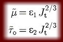
The reversible junction number J_t is directly related to the thixotropic plastic viscosity and yield value as shown with the equation below. There, the two terms ε₁ and ε₂ are material parameters depending, among other factors, on the surface roughness of the cement particles and phase volume Φ.

Model evaluation:

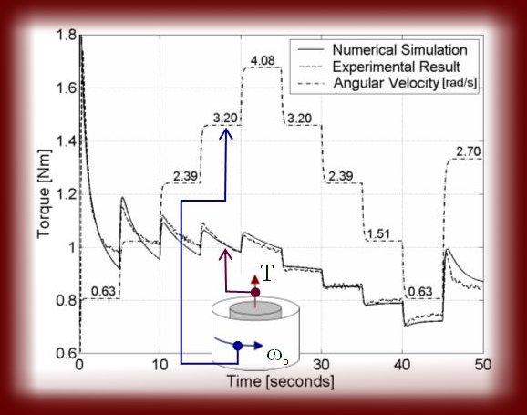
The computed torque (applied on the inner cylinder) is compared with the measured torque collected during complex shear flow. Below is an example of such comparison. As shown, the angular velocity is increasing and decreasing in steps. This is done to introduce a complicated shear rate condition, which makes simulation more difficult. With this, one can better test the quality of the proposed material model. When using a simple shear rate condition in the experiment (not done in this project), it is easy to generate a false material model, depending for example on the exponential decay of shear rate multiplied with time. Such false material model is only a shadow of the true material model, meaning if such simple shear viscosity equation is applied in another experiment of more complex shear history (like is done in this project) a failure would be certain.

Movie files of the computed results:

The simulation results shows the cement paste rheological response, when mixed with the corresponding admixture shown below. These admixtures are polymers and are designated as VHMW Na and SNF. The first one is a very high molecular weight Na-lignosulfonate. It is a natural polymer formed from the pulping process and is produced by Borregaard LignoTech, Norway. The SNF is a sulfonated naphthalene - formaldehyde condensate polymer and is synthetically formed. It has the commercial name Suparex M40 and is produced by Hodgson Chemicals Ltd.

1. Corner-flow for the VHMW Na case; Here is the relative velocity profile shown inside the ConTec Viscometer 4, at the bottom-corner (see Figure 7.1, p.156 and Figure 8.21, p.200). This is a computed flow, by the software shown below. Dark blue means zero velocity, while dark red means maximum velocity (4.08 rad/s · 10.1 cm = 41.2 cm/s). For this case, the cement paste is mixed with the VHMW Na Lignosulfonate (see Section 9.4, p.214). The time is 102 minutes after water addition.
2. Torque plotted as a function of time for the VHMW Na case; Here is both the measured and computed torque plotted as a function of time. Single experiment takes 50 seconds. Also shown, is the rotational frequency f (in revolutions per seconds) of the outer cylinder (i.e. of the bucket that contains the cement paste). As before, the cement paste is mixed with the VHMW Na Lignosulfonate and the time is 102 minutes after water addition.
3. Torque as a function of time for the SNF case; Here, the cement paste is mixed with the SNF polymer and the time is 72 minutes after water addition (see Section 9.8, p.231).

Source code:

Due to very complex material model (i.e. viscoplastic fluid with fading memory and so forth), it was more or less impossible to use commercial programs available. Hence, I had to write (in Fortran 90 - ANSI X3.198-1992; ISO/IEC 1539-1:1991 (E)) my own program, called Viscometric-ViscoPlastic-Flow (later designated as version 1.0). It consists of seven files and the newest version is listed below. Viscometric-ViscoPlastic-Flow is a free software; which can be redistributed and/or modified under the terms of the GNU General Public License as published by the Free Software Foundation; either version 2 of the License, or (at the users option) any later version (see copying). Note that this software can be downloaded (makefile included) in the download section.

1. param.f90: This code defines and sets all variables of relevance, like the radius of inner cylinder, outer cylinder, height of inner/outer cylinder, grid step, time step, tolerance and so forth.
2. motion.f90: This file reads the basic information from param.f90 to produce continuous angular velocity as a function of time. The information about the angular velocity is requested by the routine main.f90.
3. viscous.f90: In this file, the shear viscosity function η is defined and calculated. This information is requested by update.f90.
4. write2f.f90: This file takes care of writing all computed data into the different files. It is only the source main.f90 that makes such request.
5. shear.f90: This routine calculates the shear rate from the computed velocity profile. It is the program update.f90 that makes the request.
6. update.f90: This file sets up the system of algebraic equations to be solved. This file also contains the algorithm that is used in solving this system.
7. main.f90: This is the center of the whole software, holding and passing information to and from the different subroutines. Some subroutines interact directly with each other without going through the channels defined by main.f90 (this applies mostly for the subroutines in the files update.f90, shear.f90 and viscous.f90). The geometry of the viscometer, including the bottom cone, is defined in this part of the software.

BIBLIOGRAPHY

1. Wallevik, J. E. (2005); Thixotropic investigation on cement paste: Experimental and numerical approach. J. Non-Newtonian Fluid Mech. 132 (2005) 86-99.
2. Wallevik, J. E. (2004); Microstructure-Rheology: Thixotropy and Workability Loss; Nordic Concrete Research, Publication No. 31, The Nordic Concrete Federation 1/2004, Norsk Betongforening, Oslo, Norway.
3. Wallevik, J. E. (2003); Rheology of Particle Suspensions - Fresh Concrete, Mortar and Cement Paste with Various Types of Lignosulfonates (Ph.D.-thesis); Department of Structural Engineering, The Norwegian University of Science and Technology. ISBN 82-471-5566-4; ISSN 0809-103X.
4. Oldroyd, J. G. (1947); A Rational Formulation of the Equations of Plastic Flow for a Bingham Solid, Proc. Camb. Philos. Soc. Vol. 43.
5. Hattori, K. & Izumi, K. (1991), In P. F. G. Banfill (Ed.), Rheology of Fresh Cement and Concrete, Proc. of the International Conference Organized by The British Society of Rheology, University of Liverpool, 16 - 29 March 1990, E & FN Spon, London.

Height-independence in the coaxial cylinders viscometers (VVPF 1.0)

The viscometers under consideration in this project are the ConTec BML Viscometer 3 and ConTec Viscometer 4. Major figures or other results from this project will not be published on this site until in some near future.

BIBLIOGRAPHY

1. Wallevik, J. E., Minimizing end-effects in the coaxial cylinders viscometer: Viscoplastic flow inside the ConTec BML Viscometer 3. J. Non-Newtonian Fluid Mech. 155 (2008) 116-123.

Particle migration

Shear rate induced particle migration is a possibility in all types of viscometers. For further readings about this subject, see Chapter 10 (p.237) in my Ph.D. thesis "RHEOLOGY OF PARTICLE SUSPENSIONS" (see the link page, about the download location).

Sea ice rheology

This is a research project that I was involved during my employment at the Icelandic Meteorological Office. The project was under supervision of Dr. Thor E. Jakobsson. The purpose of the project was to test a specific real-time sea ice model in Icelandic waters. If successful, such model could be used to forecast the sea ice movement few days ahead for ships that are about to enter sea ice zones.

The model that was used is a Canadian real-time sea ice model called Multi Category Regional Ice Model, version 2.5 (MCRIM 2.5). The model is being developed and is run daily by the Canadian weather service AES (Atmospheric Environment Service). This model (version 2.5) solves the governing equation (i.e. Newton's second law) using Hibler's constitutive equation [1]. The conservation equation used in this model is from Thorndike et al. [2]. Below is a numerical result that shows forecast of the total ice compactness in percentages on Icelandic waters. Initial condition is taken from the 18th of January 1997 at 12:00 GMT (0 hours). From left to right and top to bottom are simulation results at 24, 72, 120 and 160 hours [3,4]. In the western region of the calculation domain, the numerical result corresponded to what was observed. It was harder to judge the remaining region, due to lack of data.

In this project, a so-called HIRLAM coordinates was used (HIRLAM = High Resolution Limited Area Model). Briefly explained, in this coordinate system the latitude and longitude coordinates are moved towards the north. This is done to be able to work with square latitude-longitude grid cells. In the above figure, the usual latitude-longitude coordinates are also shown.

The overall result from this project was that the MCRIM 2.5 worked relatively well. However, due to lack of real time ocean currents, some mismatch between the computed result and observation occurred in some cases.

Movie files of the computed results:

The duration of each simulation ("the forecast time") is one week (i.e. 168 hours) and has a start time 12:00 GMT at the corresponding day, shown below. The simulation result is of total ice compactness in percentages on Icelandic waters. As shown in the above figure, dark red means a complete coverage of sea ice, while light blue means no sea ice (i.e. open ocean). Dark blue is land mass (i.e. Iceland, Greenland and JanMayen).

1. 2nd of January 1997 (12:00 GMT);
2. 10th of January 1997 (12:00 GMT);
3. 18th of January 1997 (12:00 GMT); This is the same result as shown in the above figure.

BIBLIOGRAPHY

1. Hibler III W. D. (1977); A Viscous Sea Ice Law as a Stochastic Average of Plasticity. Journal of Geopysical Research (Vol. 82, No. 27). pp.3933-3934.
2. Thorndike A. S., Rothrock D. A., Maykut G. A. & Colony R. 1975. The Thickness Distribution of Sea Ice. Journal of Geophysical Research (Vol. 80, No. 33). pp.4501-4505.
3. Wallevik, J. E. (1999); Implementation of the Sea Ice Model MCRIM 2.5 to Icelandic Waters. The Icelandic Meteorological Office. Iceland. Report: VI-G99017-UR09 (in Icelandic).
4. Wallevik, J. E. (2003); Rheology of Particle Suspensions - Fresh Concrete, Mortar and Cement Paste with Various Types of Lignosulfonates (Ph.D.-thesis). Department of Structural Engineering, The Norwegian University of Science and Technology. ISBN 82-471-5566-4. ISSN 0809-103X

Relationship between the Bingham parameters and slump

Viscometers in general have never been particularly popular at the jobsite. They are however well suited at the laboratory as they measure concrete consistency in terms of fundamental physical quantity, known as the yield stress and plastic viscosity. In contrast to viscometers, the slump cone is by far the most accepted tool for measuring consistency at the jobsite. This is due to its simplicity in handling. With the significance of both types of devices, it is clearly important to relate them to each other. The result of this study suggests a relationship between the yield stress and slump that depends on the concrete mixture proportions. More precisely, a particular trend line between the yield stress and slump seems to depend on volume fraction of matrix used in the concrete. The study shows a low correlation between the slump and plastic viscosity.

BIBLIOGRAPHY

1. Wallevik, J. E. (2006); Relationship between the Bingham parameters and slump. Cement and Concrete Research, 36, 1214-1221.
2. Wallevik, J. E. (2003); Rheology of Particle Suspensions - Fresh Concrete, Mortar and Cement Paste with Various Types of Lignosulfonates (Ph.D.-thesis). Department of Structural Engineering, The Norwegian University of Science and Technology. ISBN 82-471-5566-4. ISSN 0809-103X